In the last post, we discussed a technique by which we can have an estimate of the size of the nucleus. We saw a graph between the differential cross-section per unit solid angle and the scattering angle obtained from an electron scattering experiment with the Carbon nucleus. We compared that graph with the single slit diffraction pattern for circular aperture and found the size of the carbon nucleus. We found the radius of the carbon nucleus to be 2.3\rm \ femtometer which is quite closer to its actual radius. But with a little bit more calculations, we can get more information about the size of the nucleus with the help of quantum mechanics.
First, let’s have a look at different methods by which we can get the size of a nucleus. These are some techniques that we can use for the measurement of the size of a nucleus.
Electromagnetic Interaction: This is the interaction between charged particles. And it’s going to tell us where the charged particle, where the protons, are inside the nucleus.
- Here, we can have a look at electron scattering or we can have a look at muonic atoms where muons are orbiting nuclei. That’s very interesting because the orbit of the muons is really quite different than the electrons orbiting nuclei.
- We can also have a look at mirror nuclei, this is where we have the same number of nucleons between two nuclei, but different numbers of protons and neutrons. And beta decay between these nuclei is very important.
Strong Interaction: It will tell us at which position all the protons and neutrons sitting inside a nucleus. Since strong interaction just tell us where the proton or the neutron is sitting inside a nucleus so to know the distribution of matter inside a nucleus we need to take into account the strong and the electromagnetic interactions at the same time.
- Here we can have a look at alpha particle scattering in which alpha particles are going to interact with the nuclei. And they are going to interact with it electromagnetically and via strong interaction.
- We can have a look at the protons and neutrons scattering and they also interact via electromagnetic and strong force.
- We can have a look at the lifetime of alpha-particle emitters.
- We can have a look at the lifetime of alpha decay which is quite interesting and tells us a lot about the size of nuclei as well.
- And we can have a look at \pi mesic X-rays.
Now with all of these different ways of having a look at the size of the nucleus, we find the radii are equal for all of these different methods. In this post, we will discuss electron scattering in detail.
Detailed Study Of Electron Scattering
Since electrons do not exert nuclear force on the nucleus. So, the interaction of electrons with the nucleus is just a Coulomb interaction and the Hamiltonian of the system can be written as
\begin{aligned}H&=H_0+V(r)\\ \end{aligned}
Where H_0 is the Hamiltonian of a free electron and V(r) is the potential energy between the electron and the nucleus due to coulomb interaction. V(r) is also called as scattering potential.
The Hamiltonian of a free electron can be written as
\begin{aligned}H_0&= \dfrac{P^2}{2m}\\ \end{aligned}
It can also be written as
\begin{aligned}H_0 &\equiv \dfrac{- \hbar^2}{2m \nabla^2}\end{aligned}
\textcolor{red}{(1)}
Where P is the momentum of the free electron and m is the mass of the electron.
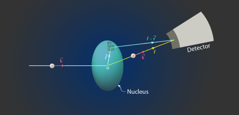
Suppose there is a nucleus in which there is a volume element d\tau which is at a position \vec{r^\prime} from the center of the nucleus and this is the electron at a position \vec r from the origin of the co-ordinate axis as shown in the diagram below. (Electrons may be anywhere in space. It can be either outside or inside the nucleus).
Let \rho(r^\prime) is the density of the nucleus at the position of the elementary volume d\tau. Then the scattering potential V(r) will be
\begin{aligned}V(r)&= \int_v \dfrac{\rho(\vec{r^\prime}) d\tau (-e)}{4\pi \epsilon_0 (\vec{r} -\vec{r^\prime})}\\ \end{aligned}
\textcolor{red}{(2)}
Consider an incident electron wave of momentum \vec{p} that is going along \vec k and after the interaction with the nucleus, its momentum becomes \vec{p^\prime} and goes along \vec {k^\prime}.
The wave function of an incident electron can be written as;
\begin{aligned}\psi_0&=e^{(i\vec{k}\cdot \vec{r})}\\\end{aligned}
Here \vec k is the wave vector whose direction is along the direction of motion of the incident electron and magnitude depends on the energy of the incident electron. It is given by;
\begin{aligned}\vec{k}&= \hbar \vec{p}\\\end{aligned}
From the quantum mechanics, we can write
\begin{aligned}H_0 \psi_0&=E\psi_0\\\end{aligned}
where E is the energy of the incident electron that can be expressed as;
\begin{aligned}E&=\dfrac{\hbar^2 k^2}{2m}\\ \end{aligned}
\textcolor{red}{(3)}
The Schrödinger’s equation for the scattering problem is;
\begin{aligned} (H_0+V(r))\psi&=E\psi\\\end{aligned}
Here \psi is the wavefunction of the electron after scattering. If we substitute the value of H_0 and E from equations 1 and 3 in the above equation then the Schrödinger’s equation for the scattering problem can also be written as;
\begin{aligned} (\nabla^2+k^2)\psi&=\dfrac{2m}{\hbar^2}V(r)\psi\\\end{aligned}
This equation is subject to the boundary condition \psi\rightarrow \psi_0\ \text{as}\ V(r)\rightarrow 0. The solution of the above equation can be obtained by comparing the solution of the Helmholtz equation and it would be like
\begin{aligned}\psi(\vec{r})&= \psi_0 (\vec{r})- \dfrac{2m}{\hbar^2}\int \dfrac{e^{ik|\vec{r}-\vec{r^\prime}|}}{4\pi|\vec{r}-\vec{r^\prime}|} V(\vec{r^\prime})\psi(\vec{r^\prime}) d^3 \vec{r^\prime}\\ \end{aligned}
\textcolor{red}{(4)}
Now let’s calculate the value of \psi(\vec{r}) well outside the scattering region. That is we want to calculate \psi(\vec{r}) for r\gg r^\prime. Since the scattering potential V(\vec{r^\prime}) is localized about r^\prime=0. That is the potential drops to zero outside of a finite region. So, for r\gg r^\prime we have
\begin{aligned}|\vec{r} -\vec{r^\prime}|^2&=(\vec{r} -\vec{r^\prime})\cdot(\vec{r} -\vec{r^\prime})\\&=r^2+(r^\prime)^2-2\vec{r}\cdot\vec{r^\prime} \\&\approx r^2 \left (1-2 \dfrac{\vec{r} \cdot\vec{r^\prime}}{r^2}\right )\\&= r^2 \left (1-2 \dfrac{\hat{r}\cdot\vec{r^\prime}}{r} \right)\\\Rightarrow |\vec{r} -\vec{r^\prime}|&= r (1-2 \left (\dfrac{\hat{r}\cdot\vec{r^\prime}}{r} \right)^{\frac{1}{2}}\\&\approx r (1-\left (\dfrac{\hat{r}\cdot\vec{r^\prime}}{r} \right)\\\Rightarrow |\vec{r} -\vec{r^\prime}|&\approx r- \hat{r}\cdot\vec{r^\prime} \\\end{aligned}
Now if we define the wave vector for scattered electron as \vec{k^\prime}=k\hat{r} because the scattered electron has almost the same energy as the incident electron then equation 4 reduces to
\begin{aligned}\psi(\vec{r}) &\approx \psi_0 (\vec{r})- \dfrac{2m}{\hbar^2}\int \dfrac{e^{ik(r- \hat{r}\cdot\vec{r^\prime})}}{4\pi|\vec{r}-\vec{r^\prime}|} V(\vec{r^\prime})\psi(\vec{r^\prime}) d^3 \vec{r^\prime}\end{aligned}
Since we have e^{ik(r- \hat{r}\cdot\vec{r^\prime})}= e^{ikr} e^{-i\vec{k^\prime}\cdot \vec{r^\prime}} and |\vec{r} -\vec{r^\prime}| \approx r so we can write
\begin{aligned}\psi(\vec{r}) &\approx e^{i\vec{k}\cdot\vec{r}}-\dfrac{e^{ikr}}{r} \dfrac{m}{2\pi\hbar^2} \int e^{-i\vec{k^\prime}\cdot\vec{r^\prime}} V(\vec{r^\prime})\psi(\vec{r^\prime}) d^3 \vec{r^\prime}\\ \end{aligned}
\textcolor{red}{(5)}
We can also write the above equation as
\begin{aligned}\psi(\vec{r} )&\approx e^{i\vec{k}\cdot\vec{r}}+\dfrac{e^{ikr}}{r} f(k,k^\prime)\\ \end{aligned}
Where e^{i\vec{k}\cdot\vec{r}} represents the incident particle beam, \dfrac{e^{ikr}}{r} is outgoing spherical wave and f(k,k^\prime) is scattering amplitude. We have
\begin{aligned}f(k,k^\prime)&= – \dfrac{m}{2\pi\hbar^2} \int e^{-i\vec{k^\prime}\cdot\vec{r^\prime}} V(\vec{r^\prime})\psi(\vec{r^\prime}) d^3 \vec{r^\prime}\\\end{aligned}
So far, we only assumed r\gg r^\prime. Now suppose that the scattering is not particularly strong. In this case, it is reasonable to suppose that the wavefunction, \psi(\vec{r}), does not differ substantially from the incident wavefunction, \psi_0 (\vec{r}). Thus, we can obtain an expression for f(k,k^\prime) by making the substitution \psi(\vec{r}) \rightarrow \psi_0 (\vec{r}) in the above equation. This procedure is a weak potential approximation which is specially called the Born approximation. So, the Born approximation yields
\begin{aligned}f(k,k^\prime ) &\approx – \dfrac{m}{2\pi\hbar^2} \int e^{i(\vec{k}-\vec{k^\prime})\cdot\vec{r^\prime}} V(\vec{r^\prime}) d^3 \vec{r^\prime}\\\end{aligned}
If we consider, \vec{q}= \vec{k^\prime}-\vec{k} then f(k,k^\prime) can be written as;
\begin{aligned}f(k,k^\prime )&\approx – \dfrac{m}{2\pi\hbar^2} \int e^{-i\vec{q}\cdot\vec{r^\prime}} V(\vec{r^\prime}) d^3 \vec{r^\prime}\\\end{aligned}
That can be further written as;
\begin{aligned}f(k,k^\prime)&\approx – \dfrac{m}{2\pi\hbar^2} \int e^{-i\vec{q}\cdot\vec{r}} V(\vec{r}) d^3 \vec{r}\\\end{aligned}
If the total nuclear charge is Ze, we can express the nuclear charge density as Ze \rho(r^\prime) .
Here \rho(r^\prime) is the charge distribution which is normalized to 1 that is we have \int \rho(r^\prime)d^3r^\prime= 1. Thus the potential energy of the electron is given by;
\begin{aligned}V(\vec{r} )&=\dfrac{-Ze^2}{4\pi\epsilon_0} \int_v \dfrac{\rho(\vec{r^\prime}) d^3 \vec{r^\prime}}{|\vec{r} -\vec{r^\prime}|}\\\end{aligned}
And by making the substitution \vec{R} =\vec{r} – \vec{r^\prime} and d^3 (\vec{r}) \approx d^3(\vec{R}) we have the integral
\begin{aligned}\int e^{-i\vec{q}\cdot\vec{r}} V(\vec{r}) d^3 \vec{r}&=\dfrac{-Ze^2}{4\pi\epsilon_0}\int e^{-i\vec{q}\cdot\vec{r}}\left [ \int_v \dfrac{\rho(\vec{r^\prime}) d^3 \vec{r^\prime}}{ |\vec{r} -\vec{r^\prime}|} \right ] d^3 \vec{r}\\ &= \dfrac{-Ze^2}{4\pi\epsilon_0}\int e^{-i\vec{q}\cdot (\vec{r^\prime}+\vec{R})}\left [ \int_v \dfrac{\rho(\vec{r^\prime}) d^3 \vec{r^\prime}}{R} \right ] d^3 \vec{R}\\ &=\left [ \dfrac{-Ze^2}{4\pi\epsilon_0}\int \dfrac{e^{-i\vec{q}\cdot\vec{R}}}{R} d^3 \vec{R} \right ] \left ( \int_v e^{-i\vec{q}\cdot \vec{r^\prime}} \rho(\vec{r^\prime}) d^3 \vec{r^\prime} \right )\\ \end{aligned}
Here the expression in the bracket [\ ] is the probability amplitude for a point-like nucleus and the expression in the bracket (\ ) is the probability amplitude for the spatial extent of the nucleus, specially called the Form Factor denoted by F(q) . So we have the formula for the Form factor and it is given by;
\begin{aligned}F(q)&= \int_v e^{-i\vec{q}\cdot \vec{r^\prime}} \rho(\vec{r^\prime}) d^3 \vec{r^\prime}\\ \end{aligned}
\textcolor{red}{(6)}
Now the differential cross-section for an extended nucleus can be written as;
\begin{aligned}\dfrac{d\sigma}{d\Omega}&=\left (\dfrac{d\sigma}{d\Omega}\right)_{point} |F(q) |^2\\\end{aligned}
So we can say, the electron scattering of an extended source is equal to the scattering of a point-like source modulated by the form factor.
From equation 6 we can say that the Form Factor is the Fourier transform of the normalized charge distribution. So, if you know the distribution of charge density in the nucleus, then you can just put it here in this integration and do all this calculation and get the cross-section. But, the problem is reversed here. We really don’t know the charge density. We don’t know how the charge is distributed in the nucleus. We only know about the total charge of the nucleus which is Ze.
Don’t worry. We can do it in a reverse way. We will discuss it in the next post.