In the previous post, we created and visualized histograms in CERN ROOT using PyROOT.
Now we’ll take the next step: fit a function to our data and extract useful quantities like
the mean, RMS, and fit parameters with uncertainties.
This is a key skill in nuclear and high-energy physics, where we often model peaks (e.g., energy lines) with
Gaussian functions to measure centroids and resolutions.
🎯 What You Will Learn
- How to write and run a PyROOT script from a .py file
- How to fit a Gaussian to a histogram
- How to read the histogram’s Mean and RMS
- How to get fit parameters and their errors
- How to save the plot image and a ROOT file with your histogram
📄 Step 1 — Create the Python File
Open a text editor (Notepad, VS Code, etc.), paste the code below, and save it as root_fit_gaussian.py.
import ROOT

# ------------------------------------------------------------
# 1) Create a histogram and fill with Gaussian random values
# ------------------------------------------------------------
ROOT.gRandom.SetSeed(12345)  # reproducible example
h = ROOT.TH1F("h", "Gaussian Example; X; Counts", 60, -4.0, 4.0)

for _ in range(12000):
    h.Fill(ROOT.gRandom.Gaus(0.0, 1.0))  # mean=0, sigma=1

# Quick sanity check: basic stats from the histogram itself
print("Histogram mean (approx):", round(h.GetMean(), 3))
print("Histogram RMS (approx):", round(h.GetRMS(), 3))

# ------------------------------------------------------------
# 2) Make a canvas and draw the histogram
# ------------------------------------------------------------
c = ROOT.gROOT.FindObject("c")
if not c:
    c = ROOT.TCanvas("c", "Gaussian Fit Demo", 900, 650)

h.SetLineColor(ROOT.kBlue + 1)
h.SetLineWidth(2)
h.SetFillColor(ROOT.kAzure - 9)
h.SetFillStyle(3004)
h.Draw()

# ------------------------------------------------------------
# 3) Fit a Gaussian to the histogram
# ------------------------------------------------------------
# "gaus" is a built-in Gaussian function in ROOT:
#   f(x) = p0 * exp( -0.5 * ((x - p1)/p2)^2 )
# where p0=amplitude, p1=mean, p2=sigma
fit_result = h.Fit("gaus", "S Q")  # "S"=store result, "Q"=quiet (no spam)

# Retrieve the fitted TF1 and parameters
f = h.GetFunction("gaus")
amp   = f.GetParameter(0); amp_err   = f.GetParError(0)
mean  = f.GetParameter(1); mean_err  = f.GetParError(1)
sigma = f.GetParameter(2); sigma_err = f.GetParError(2)

print("\\n--- Gaussian Fit Results ---")
print(f"Amplitude  = {amp:.3f} ± {amp_err:.3f}")
print(f"Mean (μ)   = {mean:.3f} ± {mean_err:.3f}")
print(f"Sigma (σ)  = {sigma:.3f} ± {sigma_err:.3f}")
print(f"Chi2/NDF   = {fit_result.Chi2():.1f} / {fit_result.Ndf()}")

# ------------------------------------------------------------
# 4) Optional: Fit only a specific range (uncomment to try)
# ------------------------------------------------------------
# h.Fit("gaus", "S Q", "", -2.0, 2.0)  # fit only the central peak region

# ------------------------------------------------------------
# 5) Polish the look and save outputs
# ------------------------------------------------------------
# Draw the fitted function in red
f.SetLineColor(ROOT.kRed + 1)
f.SetLineWidth(3)
c.Modified(); c.Update()

# Save an image
c.SaveAs("gaussian_fit.png")
print("Saved: gaussian_fit.png")

# Save to a ROOT file for later reuse
out = ROOT.TFile("gaussian_fit_output.root", "RECREATE")
h.Write()
f.Write("gaus_fit")  # save the function with a chosen name
out.Close()
print("Saved: gaussian_fit_output.root")

# Keep the canvas open if running interactively (optional):
# input("Press Enter to close...")
🔽 Detailed Explanation of the code (Click to Expand)
Show / Hide Explanation
Let’s go through some important parts of the Python code so that you understand what each section does.1️⃣ Importing ROOT
import ROOTTH1F, TCanvas, TFile, etc.)
using the prefix ROOT..
2️⃣ Creating and Filling the Histogram
ROOT.gRandom.SetSeed(12345)  # reproducible example
h = ROOT.TH1F("h", "Gaussian Example; X; Counts", 60, -4.0, 4.0)

for _ in range(12000):
h.Fill(ROOT.gRandom.Gaus(0.0, 1.0))ROOT.gRandom.SetSeed(12345): sets the random-number seed so you always get the same random data. Useful for tutorials.TH1F: creates a 1D histogram with:"h"— internal name of the histogram"Gaussian Example; X; Counts"— title and axis labels (before semicolon = title, after = X and Y labels)60— number of bins-4.0, 4.0— x-axis range
for _ in range(12000): ...: fills the histogram 12,000 times with random Gaussian values.ROOT.gRandom.Gaus(0.0, 1.0): generates a random number from a Gaussian distribution with mean = 0 and sigma = 1.
3️⃣ Getting Basic Statistics from the Histogram
print("Histogram mean (approx):", round(h.GetMean(), 3))
print("Histogram RMS (approx):", round(h.GetRMS(), 3))h.GetMean(): calculates the mean value based on the filled histogram.h.GetRMS(): gives the RMS (root mean square), which is related to the width of the distribution.round(..., 3): rounds the numbers to 3 decimal places to make the output cleaner.
4️⃣ Creating the Canvas and Drawing the Histogram
c = ROOT.gROOT.FindObject("c")
if not c:
    c = ROOT.TCanvas("c", "Gaussian Fit Demo", 900, 650)

h.SetLineColor(ROOT.kBlue + 1)
h.SetLineWidth(2)
h.SetFillColor(ROOT.kAzure - 9)
h.SetFillStyle(3004)
h.Draw()gROOT.FindObject("c"): if a canvas named"c"already exists (e.g., from a previous run), reuse it.- Otherwise,
TCanvas("c", "Gaussian Fit Demo", 900, 650)creates a new window of size 900×650 pixels. SetLineColor,SetFillColor,SetFillStyle: change how the histogram looks (line color, fill color, pattern).h.Draw(): actually draws the histogram on the current canvas.
5️⃣ Fitting a Gaussian to the Histogram
fit_result = h.Fit("gaus", "S Q")  # "S"=store result, "Q"=quiet (no spam)

f = h.GetFunction("gaus")
amp   = f.GetParameter(0); amp_err   = f.GetParError(0)
mean  = f.GetParameter(1); mean_err  = f.GetParError(1)
sigma = f.GetParameter(2); sigma_err = f.GetParError(2)
h.Fit("gaus", "S Q"):"gaus"— tells ROOT to use its built-in Gaussian function."S"— store the fit result in aTFitResultPtrobject (fit_result)."Q"— quiet mode (do not print a long fit report to the terminal).
h.GetFunction("gaus"): gets the fitted function object (aTF1).GetParameter(i): returns parameteri:- 0 → amplitude (height of the peak)
- 1 → mean (μ), position of the peak
- 2 → sigma (σ), width of the peak
GetParError(i): gives the uncertainty (error) on parameteri.
6️⃣ Checking Fit Quality: Chi2/NDF
print(f"Chi2/NDF = {fit_result.Chi2():.1f} / {fit_result.Ndf()}")fit_result.Chi2(): the χ² value of the fit.fit_result.Ndf(): number of degrees of freedom.Chi2/NDFnear ~1 often indicates a reasonable fit (but always check the plot visually).
7️⃣ Saving the Plot as an Image
c.SaveAs("gaussian_fit.png")
print("Saved: gaussian_fit.png")SaveAs("gaussian_fit.png"): saves whatever is currently drawn on the canvas to a PNG file.- You can also use other formats:
.pdf,.root,.jpg, etc.
8️⃣ Saving the Histogram and Fit to a ROOT File
out = ROOT.TFile("gaussian_fit_output.root", "RECREATE")
h.Write()
f.Write("gaus_fit")
out.Close()
TFile("gaussian_fit_output.root", "RECREATE"): opens a ROOT file in “recreate” mode (overwrite if it exists).h.Write(): stores the histogram inside the ROOT file.f.Write("gaus_fit"): stores the fitted function with the name"gaus_fit".out.Close(): closes the file and writes everything to disk.
▶️ Step 2 — Run the Script in the ROOT Environment
Open a command prompt with ROOT environment configured:
cd C:\root\root\bin
thisroot.bat
Now run your Python script (using the same Python version you installed for ROOT):
py -3.11 C:\root\root\bin\root_fit_gaussian.py(In my computer, the path of the folder where the code root_fit_gaussian.py is saved is C:\root\root\bin. You have to choose your folder path.)
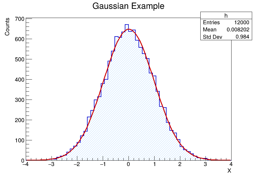
You should see printed results in the console and two files in your working directory:
gaussian_fit.png— the plot with the fitted curve as shown belowgaussian_fit_output.root— a ROOT file containing the histogram and the fit function
🔍 Understanding the Output
- Mean (μ) — position of the peak (centroid)
- Sigma (σ) — width (standard deviation). In detector spectra, this relates to resolution.
- Chi2/NDF — goodness of fit. Values near ~1 are typically “reasonable,” but always check residuals.
🧰 Useful Variations (Try These)
- Change the fill:
h.SetFillStyle(0)to turn off shading - Change the fit range: uncomment the example fit command with limits
- Use a custom function:
# Example of a custom Gaussian (same shape as "gaus")
custom = ROOT.TF1("custom", "[0]*exp(-0.5*((x-[1])/[2])**2)", -4, 4)
custom.SetParameters(500, 0.0, 1.0)  # initial guesses
h.Fit(custom, "S Q")
🧭 Troubleshooting
- NameError: name ‘c’ is not defined — make sure you created the canvas:
c = ROOT.TCanvas(...) - import ROOT fails — you forgot to run
thisroot.batfirst in that terminal - Fit looks bad — try limiting the fit range to around the peak; check binning and statistics
- No image saved — ensure you called
c.SaveAs("...")after drawing
📚 What’s Next?
In the next post, we’ll learn how to build 2D histograms (TH2F),
draw density/colz plots, and visualize correlations between two variables—very useful for
coincidence studies and detector calibrations.
References & Further Reading
- CERN ROOT — Official Website: https://root.cern/
- Brun, R. & Rademakers, F. (1997). “ROOT – An Object Oriented Data Analysis Framework.” Nuclear Instruments and Methods in Physics Research A, 389(1–2), 81–86. DOI: 10.1016/S0168-9002(97)00048-X
- CERN Documentation: ROOT User Manual and Tutorials
- TMVA Toolkit for Multivariate Data Analysis: https://root.cern/manual/tmva/
- GEANT4 Collaboration. “GEANT4 – A Simulation Toolkit.” Nuclear Instruments and Methods in Physics Research A, 506(3), 250–303 (2003). DOI: 10.1016/S0168-9002(03)01368-8
- FLUKA Simulation Package — Official CERN Page: https://fluka.cern/
- CERN Open Data Portal — Public Datasets for Education and Research: https://opendata.cern.ch/
- CERN Scientific Computing Documentation: https://home.cern/science/computing
- C++ ROOT Tutorials for Beginners (Official GitHub Examples): https://github.com/root-project/root/tree/master/tutorials