Theory:
Before directly going to the program, let’s have an overview of the Fourier terms of the triangular wave.
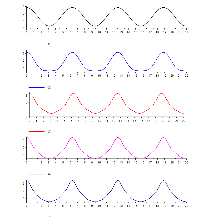
The Fourier series of the triangular waves is given by
\begin{aligned}f(x) &= \dfrac{\pi}{2}+\dfrac{\pi}{4} \sum_{n=0}^{\infty}\dfrac{1}{n^2} \cos (nx)\\\end{aligned}
From the above Fourier series, the partial sum of the first term is
S_1 = \dfrac{\pi}{2}+\dfrac{\pi}{4} \times \cos x
The partial sum of the first two terms is
\begin{aligned}S_2 &= \dfrac{\pi}{2}+\dfrac{\pi}{4} \left( \cos x +\dfrac{1}{2^2} \cos 2x \right) \\\end{aligned}
The partial sum of the first three terms is
\begin{aligned}S_3 &= \dfrac{\pi}{2}+\dfrac{\pi}{4} \left ( \cos x +\dfrac{1}{2^2} \cos 2x +\dfrac{1}{3^2} \cos 3x \right ) \\\end{aligned}
The partial sum of the first four terms is
\begin{aligned}S_4 &= \dfrac{\pi}{2}+\dfrac{\pi}{4} \left ( \cos x +\dfrac{1}{2^2} \cos 2x +\dfrac{1}{3^2} \cos 3x +\dfrac{1}{4^2} \cos 4x \right ) \\\end{aligned}
The partial sum of the first five terms is
\begin{aligned}S_5 &= \dfrac{\pi}{2}+\dfrac{\pi}{4} \left ( \cos x +\dfrac{1}{2^2} \cos 2x +\dfrac{1}{3^2} \cos 3x +\dfrac{1}{4^2} \cos 4x +\dfrac{1}{5^2} \cos 5x \right ) \\\end{aligned}
A Program in Scilab for the Triangular Wave
Now let’s go to the program and see the triangular wave in the output. Since we have discussed a lot about how to write a program in Scilab so I am going to show you the program which I have already written for it.
Here it is.
Decoding:
Let’s explain each line of this program one by one.
- In line no. 1, command clf(); is used to erase the previous plot in the graphic window.
- Line no. 2 is written for the loop over x from x = 0 to x = 5\pi with step size 0.01.
- Line no. 3 is written for S1 which is the sum of one term of a triangular wave.
- Line no. 4 is written for S2 which is the sum of the first two terms of a triangular wave. And in the same way, the fourth, fifth, and sixth lines have been written for S3, S4, and S5 which are the sum of the first three terms, the first four terms, and the first five terms respectively.
- In Line no. 5, a subplot command is used. This command is used to break the window into m rows and n columns with position P. In this line, I have written 5 1 1 in the bracket just after the subplot. It means that the window will break into 5 rows and one column with the position at the top.
- In Line no. 9, a plot2d command is used for the graph of S1. This command is used for the plotting of the graph in two dimensions.
- In Line no. 10, a subplot command is used to break the window into 5 rows and 1 column with the position at the second place from the top.
- In Line no. 11, the plot2d command is used for the graph of S2.
- Subplot and plot2d commands are repeated for S3, S4, and S5 in the rest of the lines.
- 1, 2, 5, 6, and 9 written in lines 8, 10, 12, 14, and 16 are for the different colors of the graphs.
I hope you can understand this program in a better way. Now, let’s execute the program and see the output. Wow, it looks great.
Output