Building and Visualizing 2D Histograms in CERN ROOT (TH2F)

In the previous tutorials, you learned how to create 1D histograms and perform Gaussian fits using PyROOT.
Now we move one step ahead and explore 2D histograms, which are extremely useful in physics
for visualizing correlations between two variables — for example:

• Energy vs Time
• X vs Y detector positions
• Two correlated detector signals
• Calibration maps

In ROOT, 2D histograms are created using the TH2F class.
We will learn how to build, visualize, customize, and save them using Python.

📄 Step 1 — Create a Python Script

Open a text editor and save the following code as:
root_2d_histogram.py

import ROOT
import math
import random

# -------------------------------------------------------
# 1) Create a 2D histogram TH2F
# -------------------------------------------------------
h2 = ROOT.TH2F("h2", "2D Correlation; X values; Y values", 
               50, -4, 4,     # X bins, range
               50, -4, 4)     # Y bins, range

# -------------------------------------------------------
# 2) Fill histogram with correlated data
# -------------------------------------------------------
for _ in range(20000):
    x = ROOT.gRandom.Gaus(0, 1)
    y = 0.6 * x + ROOT.gRandom.Gaus(0, 1)  # correlation
    h2.Fill(x, y)

# -------------------------------------------------------
# 3) Create a canvas and draw the histogram
# -------------------------------------------------------
c = ROOT.TCanvas("c", "2D Histogram Example", 900, 700)
c.Divide(1, 2)

# Draw as color (heatmap)
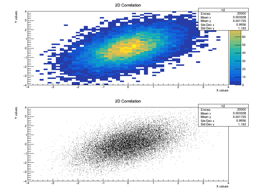
c.cd(1)
h2.Draw("COLZ")

# Draw as scatter plot
c.cd(2)
h2.Draw("SCAT")

# -------------------------------------------------------
# 4) Save the images
# -------------------------------------------------------
c.SaveAs("hist_2d_output.png")
print("Saved: hist_2d_output.png")

# Save to a ROOT file
f = ROOT.TFile("hist_2d_output.root", "RECREATE")
h2.Write()
f.Close()
print("Saved: hist_2d_output.root")

▶️ Step 2 — Run the Script

Open a ROOT-enabled terminal:

cd C:\root\root\bin
thisroot.bat

Now run your Python script:

py -3.11 C:\root\root\bin\root_2d_histogram.py

(In my computer, the path of the folder where the code root_2d_histogram.py is saved is C:\root\root\bin. You have to choose your folder path.)

You will get:

• hist_2d_output.png — the 2D plot as shown below
• hist_2d_output.root — histogram stored for later use