In the previous tutorial, we learned how to install and test CERN ROOT on Windows.
In this post, we’ll take our first practical step in data analysis — creating histograms
and visualizing data using PyROOT.
🧠 What Is a Histogram in ROOT?
A histogram is a graphical representation of data distribution.
In nuclear and particle physics, histograms are essential for displaying quantities like
energy spectra, timing distributions, or multiplicities. ROOT provides powerful classes likeTH1F (1D float histogram) and TH2F (2D float histogram)
to store and visualize such data.
🚀 Step 1 — Import ROOT and Create a Histogram
Let’s start by importing ROOT and creating a simple 1D histogram with 50 bins ranging from -4 to +4.
import ROOT

# Create a 1D histogram
h = ROOT.TH1F("h", "Gaussian Distribution; X values; Counts", 50, -4, 4)
The arguments mean:
"h"— internal name of the histogram"Gaussian Distribution; X values; Counts"— title and axis labels (separated by semicolons)50— number of bins-4, 4— x-axis range
🎲 Step 2 — Fill the Histogram with Random Data
ROOT provides a built-in random number generator, ROOT.gRandom.
Let’s fill our histogram with 10,000 Gaussian-distributed values.
for _ in range(10000):
    h.Fill(ROOT.gRandom.Gaus())
🖥️ Step 3 — Draw the Histogram on a Canvas
To visualize the histogram, create a TCanvas (ROOT’s drawing area) and use Draw().
c = ROOT.TCanvas("c", "Histogram Example", 800, 600)
h.Draw()
c.SaveAs("gaussian_hist.png")
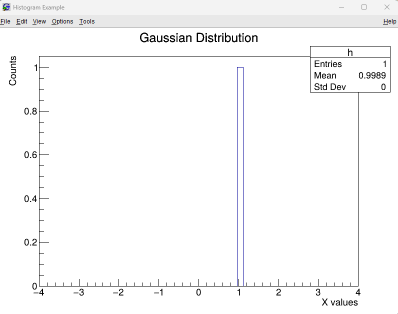
The file gaussian_hist.png will be saved in your working directory.
You can also use c.Draw() in an interactive environment to display it directly.
The histogram shown in the picture below is what you will see after this step.
🎨 Step 4 — Customize Colors and Styles
ROOT allows you to change colors, fill styles, and line thicknesses easily.
h.SetLineColor(ROOT.kBlue)
h.SetLineWidth(2)
h.SetFillColor(ROOT.kAzure - 9)
h.SetFillStyle(3004)
c.Modified()
c.Update()
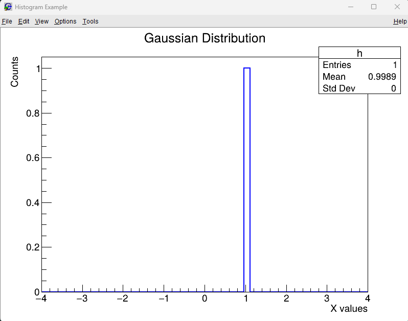
c.SaveAs("gaussian_hist_style.png")
This version will produce a more visually appealing plot with blue outlines and shaded fills (as shown below).
📁 Step 5 — Save and Reopen Histograms
You can save your histogram to a ROOT file and reload it later:
# Save to a ROOT file
f = ROOT.TFile("histogram_output.root", "RECREATE")
h.Write()
f.Close()

# Reopen and retrieve
f2 = ROOT.TFile("histogram_output.root")
h2 = f2.Get("h")
h2.Draw()
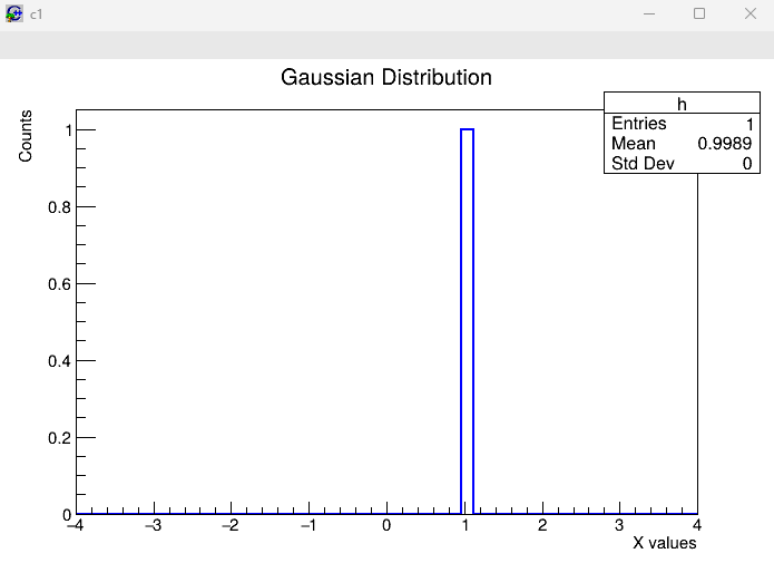
This feature is extremely useful in large experiments, where thousands of histograms are generated during detector calibration or analysis runs. Here is the output histogram with name c1.
🔽 Detailed Explanation of the code (Click to Expand)
Show / Hide Explanation
This section explains the most important lines of the histogram code so that students using CERN ROOT for the first time can clearly understand what is happening behind the scenes.1️⃣ Importing the ROOT Library
import ROOTTH1F, TCanvas, TGraph, TFile, etc. —
by writing ROOT.ClassName.
2️⃣ Creating a Histogram
h = ROOT.TH1F("h", "Gaussian Distribution; X values; Counts", 50, -4, 4)"h"— internal name (like a variable name inside a ROOT file)"Gaussian Distribution; X values; Counts"— plot title and axis labels • Before first;→ Title • Between;→ X-axis label • After last;→ Y-axis label50— number of bins-4, 4— minimum and maximum X-axis values
3️⃣ Filling the Histogram with Data
for _ in range(10000):
h.Fill(ROOT.gRandom.Gaus())ROOT.gRandom.Gaus()generates one random number from a Gaussian distribution.h.Fill(value)adds that number into the correct histogram bin.- The loop runs 10,000 times → the histogram becomes smooth and resembles a bell curve.
4️⃣ Creating a Canvas
c = ROOT.TCanvas("c", "Test Canvas", 800, 600)TCanvas in ROOT is like a blank sheet of paper — this is where ROOT draws graphs, histograms, or fits.
"c"— canvas internal name"Test Canvas"— window title800, 600— width and height in pixels
5️⃣ Drawing the Histogram
h.Draw()6️⃣ Saving the Plot as an Image
c.SaveAs("gaussian_hist.png")- You can also use other formats:
.pdf,.jpg,.eps, etc. - If the file does not appear, check that you called
Draw()beforeSaveAs().
7️⃣ Summary for Students
TH1F→ 1D histogram classFill()→ add values to the histogram binsTCanvas→ drawing surface for plotsDraw()→ draw the histogramSaveAs()→ save the plot to a file
📚 Summary
TH1Fis used for 1D histograms.- Use
Fill()to add data points. TCanvasdisplays your histogram and saves it as an image.- You can easily customize and save your histograms using ROOT’s built-in methods.
In the next blog, we’ll learn about 2D histograms (TH2F)
and how to visualize correlations between two variables.
References & Further Reading
- CERN ROOT — Official Website: https://root.cern/
- Brun, R. & Rademakers, F. (1997). “ROOT – An Object Oriented Data Analysis Framework.” Nuclear Instruments and Methods in Physics Research A, 389(1–2), 81–86. DOI: 10.1016/S0168-9002(97)00048-X
- CERN Documentation: ROOT User Manual and Tutorials
- TMVA Toolkit for Multivariate Data Analysis: https://root.cern/manual/tmva/
- GEANT4 Collaboration. “GEANT4 – A Simulation Toolkit.” Nuclear Instruments and Methods in Physics Research A, 506(3), 250–303 (2003). DOI: 10.1016/S0168-9002(03)01368-8
- FLUKA Simulation Package — Official CERN Page: https://fluka.cern/
- CERN Open Data Portal — Public Datasets for Education and Research: https://opendata.cern.ch/
- CERN Scientific Computing Documentation: https://home.cern/science/computing
- C++ ROOT Tutorials for Beginners (Official GitHub Examples): https://github.com/root-project/root/tree/master/tutorials