In the last post on nuclear physics, we derived the expression for the form factor and found that the scattering cross-section of an extended nucleus can be obtained by using the expression;
\begin{aligned}\dfrac{d\sigma}{d\Omega}&=\left (\dfrac{d\sigma}{d\Omega}\right)_{point} |F(q) |^2\\\end{aligned}
Where F(q) is the Form factor and it is given by;
\begin{aligned}F(q)&= \int_v e^{-i\vec{q}\cdot \vec{r^\prime}} \rho(\vec{r^\prime}) d^3 \vec{r^\prime}\\ \end{aligned}
Here the right side of this equation is the Fourier transforms of \rho(\vec{r^\prime}). So we can say that the Form Factor is the Fourier transforms of the normalized charge distribution.
Now, suppose, if you know the distribution of charge density in the nucleus, then you can just put it here in the above integration, do all this calculation and you can get the value of cross-section. But, the problem is reverse here. We really don’t know the charge density? We don’t know how the charge is distributed in the nucleus? We only know about the total charge of the nucleus which is Ze. So what to do? How to solve this problem? Actually, we can do it in a reverse way.
If we measure the cross-section, then we can calculate the value of the Form Factor. And from the value of the Form Factor, we can measure the charge distribution with the help of Fourier transformation.
So, what we need to do is we need to have data that we can get from experiments. Keeping this thing in mind many-electron scattering experiments were performed. Robert Hofstadter and Beat Hahn were some of them who performed experiments at Stanford University, California and they published their results in the journal Physics Review in 1953 and 1956 respectively.
In order to explicitly invert the Form Factor using the Fourier transform, a complete measure of \dfrac{d\sigma}{d\Omega} is required. But it’s very difficult to measure the differential cross-section at large deflection angles and hence fits and approximations are often used to fill in the missing data.
In the case of the spherically symmetric assumption, the resulting charge distribution is known as the Fermi model. This is defined as
\begin{aligned}\rho_c&= \dfrac{\rho_1}{1+e^{\frac{r-R}{a}}}\\\end{aligned}
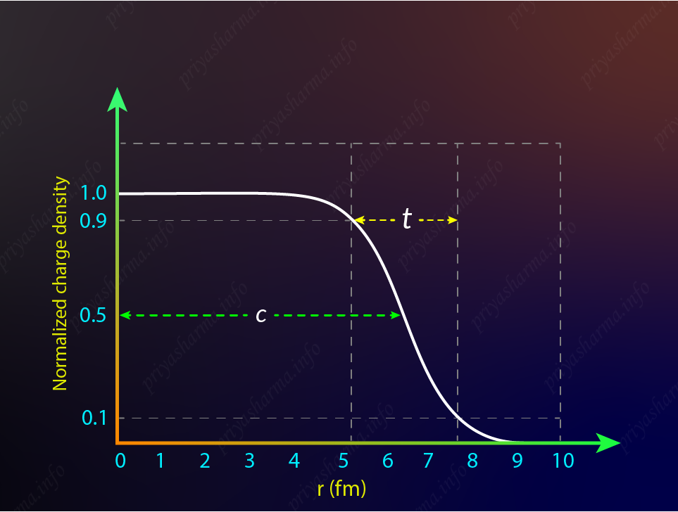
A picture of the Fermi model is shown in the above diagram. It was presented by Hofstadter in one of his lectures in 1961. The Fermi model has two parameters that can be used to describe its shape. The first parameter is c, which is the radius of the charge distribution at 50 \% of the charge density. It is called the radial parameter or half-density radius. The second parameter is a, which is related to the skin thickness t as t = (4 \ln{3})a. The ‘skin thickness’ t is the radial distance between the point of 90 \% charge density and 10 \% charge density.
Look at the picture below which is taken from the same article. This is the graph between charge density and the distance from the center of the nucleus for these different nuclei. Here you can see that the nuclear charge density or you can say proton density is constant from the center of the nucleus and up to some point and then it decreases. You can call either charged density or proton density because only protons have charge. You can also see that lighter nuclei have more charge density at the center compared to heavier nuclei. But the difference is not very much.
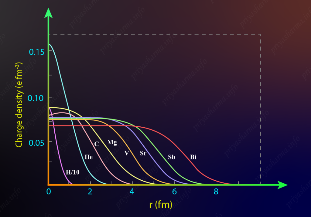
Since electrons interact only with the protons so, from this graph you can have the idea of the distribution of protons inside the nucleus. But, what is about the neutrons? Since the distribution of neutrons is almost similar to protons. So, the mass density of the nucleus can be expressed as
\begin{aligned}\rho_m&=ρ_c (\frac{A}{Z})\\&=\dfrac{\rho_1(\frac{A}{Z})}{1+e^{\frac{r-R}{a}}}\\&= \dfrac{\rho_0}{1+e^{\frac{r-R}{a}}}\\\end{aligned}
Since \dfrac{A}{Z} is different for different nuclei so, if you multiply charge density by this \dfrac{A}{Z} and try to get the total mass distribution then you find that the mass density at the center is almost same for all nuclei.
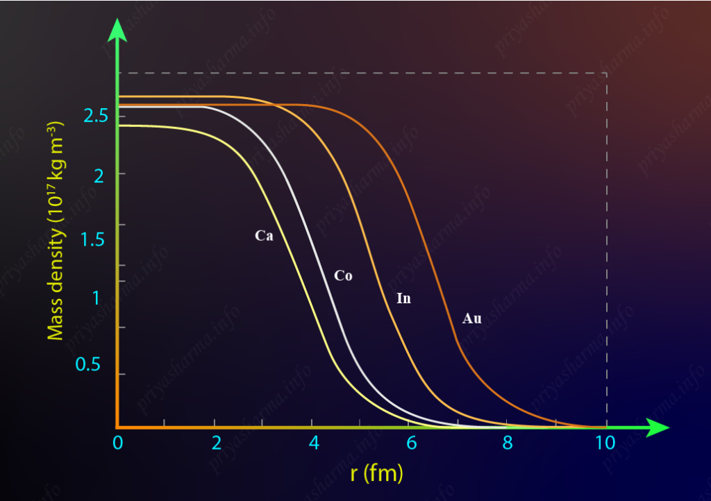
A graph of mass distribution for different nuclei is shown in the diagram below. The mass density is almost uniform from the center of the nucleus to a little bit closer to the surface and then this density gradually decreases. That, means nuclei don’t have a sharp boundary. And it could not be, because the nucleus is a quantum system.
The parameter a is found to be 0.524\rm \ fm which is approximately the same for all nuclei. And from the expression t = (4 \ln{3})a, we can get t= 2.3\rm \ fm. The parameter R is found to be some constant times A^{\frac{1}{3}}. It is given by;
\begin{aligned}R&= R_0 A^{\frac{1}{3}}\end{aligned}
where R_0 is 1.2\rm \ fm. It is the radius of Hydrogen nucleus. So, if you plug these parameters in the equation ye can find that \rho_0 is also almost 0.17\rm \ nucleons/fm^3 for all nuclei.
Conclusion:
- The density of nucleons in the core is also almost the same; whether we are talking of light nuclei or middle weight nuclei or heavyweight nuclei.
- The core size of the heavier nuclei will be larger while for the lighter nuclei, the core size will be smaller.
- The surface thickness t of the nuclei is around 2.3\rm \ fm and it is the same for almost all nuclei.