Plotting Data with TGraph & TGraphErrors in CERN ROOT

In previous posts, you learned how to build 1D and 2D histograms in ROOT.
Now we will learn a very important skill used in almost every experiment:
plotting data points, with or without error bars.

ROOT provides two common classes for this:

• TGraph — draw X–Y data points
• TGraphErrors — draw points with error bars

These are used widely in nuclear and high-energy physics for:

• Energy calibration curves
• Detector efficiency vs energy
• Reaction cross-section vs angle
• Time calibration (TDC channel vs time)

📄 Step 1 — Create a Python Script

Save the following as: tgraph_example.py

import ROOT
import math

# -------------------------------------------------------
# Example data (simulated measurements)
# -------------------------------------------------------
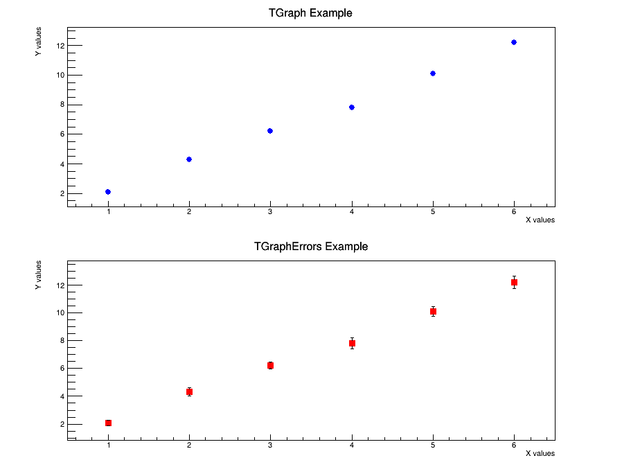
x_values = [1, 2, 3, 4, 5, 6]
y_values = [2.1, 4.3, 6.2, 7.8, 10.1, 12.2]

# Errors (optional)
y_errors = [0.2, 0.3, 0.25, 0.4, 0.35, 0.45]

# -------------------------------------------------------
# 1) Create a TGraph for simple X–Y data
# -------------------------------------------------------
graph = ROOT.TGraph(len(x_values))

for i in range(len(x_values)):
    graph.SetPoint(i, x_values[i], y_values[i])

graph.SetTitle("TGraph Example; X values; Y values")

# -------------------------------------------------------
# 2) Create a TGraphErrors for data with uncertainties
# -------------------------------------------------------
graph_err = ROOT.TGraphErrors(len(x_values))

for i in range(len(x_values)):
    graph_err.SetPoint(i, x_values[i], y_values[i])
    graph_err.SetPointError(i, 0.0, y_errors[i])  # No X error, only Y error

graph_err.SetTitle("TGraphErrors Example; X values; Y values")

# -------------------------------------------------------
# 3) Draw both graphs on a canvas
# -------------------------------------------------------
c = ROOT.TCanvas("c", "Graph Examples", 900, 700)
c.Divide(1, 2)

# Simple graph
c.cd(1)
graph.SetMarkerStyle(20)
graph.SetMarkerColor(ROOT.kBlue)
graph.Draw("AP")  # A = axes, P = points

# Graph with errors
c.cd(2)
graph_err.SetMarkerStyle(21)
graph_err.SetMarkerColor(ROOT.kRed)
graph_err.Draw("AP")  # automatically draws error bars

# -------------------------------------------------------
# 4) Save the canvas
# -------------------------------------------------------
c.SaveAs("tgraph_examples.png")
print("Saved: tgraph_examples.png")

▶️ Step 2 — Run the Script

cd C:\root\root\bin
thisroot.bat
py -3.11 C:\root\root\bin\root_2d_histogram.py

(In my computer, the path of the folder where the code root_2d_histogram.py is saved is C:\root\root\bin. You have to choose your folder path.)

You will get a two-panel plot showing:

• Simple X–Y points
• Data with error bars